Many institutional investors (not to mention many Americans interested in expanding a home or building a deck) are wondering why lumber prices have soared in 2021 – especially when raw timber has not. (“Lumber prices soar, but logs are still dirt cheap”1). Indeed, lumber prices have reached record highs at levels perhaps four times what were previously thought to be “trend” prices.
So why are lumber prices so high? And why haven’t timber prices, especially in the U.S. South, followed suit?
This article provides insights on these questions from Gwen Busby, PhD, Head of Natural Capital Research and Strategy, Nuveen, and Clark Binkley, PhD, Managing Director for International Forestry Investment Advisors located in Vancouver, Washington.
First, why did lumber prices spike?
Lumber prices actually started dropping in 2005 as housing starts fell from the record 2.2 million that year. They plummeted after the Global Financial Crisis (GFC) in 2008 then rose only slowly from the 2009 bottoms. A brief spike in 2018 was quickly extinguished by production bumps until COVID-19 hit. Though the forest sector was considered an “essential” industry, in Spring and Summer of 2020 sawmill operators struggled to maintain production. In April 2020, an estimated 35% of North American lumber capacity was down.2Strategic thinking in the industry was that demand for lumber would plummet because of the prolonged closures and restricted economic activity. All of these factors led sawmills to let lumber inventories shrink.
Then homeowners defied expectations
Developments on the demand side were precisely the opposite of what the industry anticipated, however. Many homeowners had bank accounts padded by stimulus checks and savings from foregoing normal spending during the pandemic. The homebound found joy in “repair and remodeling”: building home offices, constructing additions, and improving outdoor spaces with decking. Suddenly lumber yards faced unprecedented demand. Exploding lumber prices resulted as dealers paid panic-induced prices to fill orders.This combination of strong demand and constrained supply caused lumber prices to skyrocket from near trend levels to new record levels in the South and Pacific Northwest (PNW).

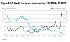
While forest owners benefited from rising timber prices in the PNW, timber prices remained subdued in the South. In 3Q 2020, just as lumber prices hit their historic high, average South-wide timber prices sank to an historic low.3
To understand what is driving the relationship between timber and lumber prices, we must explore their historical correlation, the derived demand for timber, and, finally, the ratio of timber harvest and inventory as an indicator of supply-demand balance in timber markets.
The historical correlations of lumber and timber prices
Unique market conditions in the South and PNW after the GFC led to different developments in lumber and timber markets. As shown in Figures 1 and 2, lumber and timber prices in both the South and PNW started to fall after the peak housing demand in 2005.In the South, however, the GFC reinforced the downward pressure and sawtimber prices have stayed low ever since, reaching an historic low in 3Q 2020.3 Indeed, on trend, real sawlog prices have fallen at 1.0% per year since 2000.
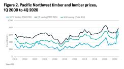
In the PNW, log prices for the two principal species – Douglas fir and “white woods” (primarily Western Hemlock) – have roughly followed lumber prices. The correlations between lumber prices and log prices are 0.65 for the pre-GFC recovery period, for the post-recovery period and, a bit tautologically, for the entire period since 2000.
Clearly, circumstances in the PNW differ materially from those in the South. But what explains the differences? More importantly, what are the implications for timberland investors?
To answer this, we must first look at the demand dynamics for lumber and timber.
Lumber demand drives timber demand
The residential construction sector – including both new housing and repair and remodeling – is the most important driver of wood products consumption in the U.S. Simply, demand for timber derives from consumer demand for lumber. Understanding the dynamics of timber demand from sawmills and supply from forest owners aids the understanding changes in timber prices.Many factors determine lumber demand, including housing starts, repair and remodeling (R&R) expenditures, and overall industrial activity. Collectively, these factors set the overall level of demand. The lumber demand curve represents the quantity of lumber demanded at every price. In short, the location of the lumber demand curve is set by the larger macro factors, but the slope is set by of the response of consumers to changes in prices.
The demand for timber is derived from the demand for lumber via the intermediary of the supply of manufacturing services. The capacity of the sawmill to pay for logs is just the price of lumber less the cost of manufacturing that lumber.4
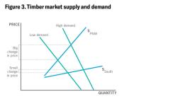
Whittling the analysis down to timber supply and demand, Figure 3 depicts two cases: one with low demand for lumber and therefore for timber (like the immediate post-GFC period) and one with high demand for lumber and therefore for timber (as seen in the current housing boom).
Figure 3 also shows timber-supply situations in two different regions; one for the PNW and one for the South. These supply curves are drawn with malice of forethought, in that supply is currently indeed flat in the South and steeper in the PNW. Increases in demand are more readily transmitted into increased in timber prices in the PNW than in the South (this works in the opposite direction as well; reductions in lumber demand translate into reductions in timber prices more rapidly in the PNW than the South).
The empirical evidence supports the way the timber supply curves are depicted in Figure 3. Using the Equation 1, we estimate the timber supply equations for the two regions and three species (in total three equations) over the period 2000-2020, with results described in Table 1.
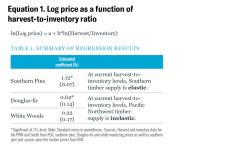
The estimated coefficients in Table 1, together with the current harvest-to-inventory ratio (H/I), tell us about the shape of the supply curve and price elasticity – or the percentage change in the quantity supplied created by a 1% change in price.
In the PNW, a change in harvest level is less than the change in price – the supply curve is steeper as drawn. In contrast, in the South, the harvest level actually changes more than the change in price.
Estimating supply-demand balance using the H/I ratio
Why are the two regions so different? Timber price is commonly modelled as a function of the H/I ratio.This makes intuitive sense – consider used cars. One dealer has a single car on the lot; a second has 1,000. If only one person shows up at each lot once, the second dealer is far more likely to give you a better price than the first. So it is with timber; if a region has a lot of timber inventory in comparison to the demand for it, many sellers will be competing for that demand, driving the price down. The opposite is also true; if demand is tight in comparison with inventory, timber prices are likely to rise.
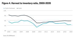
The standard for what comprises “right” and “excess” supply depends on many factors, but an important benchmark is the “normal” H/I ratio in a sustained-yield forest. Fortunately, Joseph Nikolaus von Mantel, the 19th century head of the Bavarian Forest Service, figured this out. In a sustained yield forest, the steady state H/I equals 2/T where T is the rotation age.5 In the South, a typical rotation age is 25 years, so we would expect H/I should be 8% per year; in the PNW a typical rotation age is 40 years so here we would expect H/I to be about 5% per year. In Figure 4, we plot the historical H/I ratio for the U.S. South and the PNW.
As shown in Figure 4, prior to about 2005, the ratio of H/I was around the expected values in both regions. However, in 2005 housing starts peaked at 2.2 million units and wood products demand started falling. With the precipitous decline in harvests following the GFC, the ratio of H/I declined in both regions. But in the PNW H/I rebounded sharply on the back of the increased harvest levels needed to service strong Asian log export markets. For the PNW, H/I rose through 2013 and returned to its expected level and has stayed there since.
This good fortune has eluded the South
The story in the South is quite different. Post-GFC, sawmill capacity in the South fell by almost half. Smaller, less efficient mills closed for good. Lumber demand gradually strengthened, but there was not sufficient mill capacity to translate higher lumber demand into higher demand for timber. And, to make matter worse (from the perspective of timber owners), the mills that remained post-GFC were necessarily more efficient. They used less timber per unit of lumber, dampening the demand for timber.As the Southern industry recapitalized, it did so with fewer mills that were much larger and more efficient, locking in the higher regional “lumber recovery factor” (LRF). Not only did this structural change reduce the demand for timber per unit of lumber demand, but it also resulted in fewer buyers for any specific timber tract.
Other problems plagued recovery of timber prices in the South. Government subsidies supported a planting boom in the 1980s, and that timber matured just after the GFC. Improved genetics and intensification of forest management produced yield gains in the range of 1% to 3% per year. Those productivity improvements seem small but add great volume over decades. And, to worsen matters, many landowners deferred harvests, “storing timber on the stump,” awaiting higher prices. However, this merely added to the inventory surplus.
Why Southern timber prices are still down
In summary, timber prices in the South cannot increase until the harvest-to-inventory ratio returns to its steady-state level of around 8% per year. Either harvest levels must increase and/or timber inventories must decline.Inventory will continue to increase as long as harvests are less than growth; today’s under-harvest creates tomorrow’s inventory surplus. Given the delayed development of additional sawmill capacity in the South, harvests are likely to remain below growth for a considerable period.
Harvests can’t increase until manufacturing capacity expands, either via adding shifts to mills or building new mills. Both are happening, but slowly. Adding shifts is constrained by labor supply and competition from other employers. New also mills face long waits for equipment.
Further, capacity expansion is a mixed blessing for timberland owners. Increased capacity at individual mill sites means fewer buyers for timber. Concentration in the industry reduces competition for individual timber sales. The new capacity means less additional timber demand for each unit of increased lumber demand. This latter factor has been profound, with the least efficient mills pre-GFC requiring perhaps six tons of logs per thousand board feet of lumber, while the best new capacity might require less than four tons.
What could cause timber inventory to decline in the South?
Given increased harvest levels won’t bring back balance alone, as mentioned the only other option is decreased timber inventories. However, only many years of strong demand will cause this. As seen in Figure 4, the region has been under-harvested for at least 15 years, so one might imagine a similar period of strong harvests will be required to right the balance.Of course, other factors can deplete the Southern timber inventory, such as drought, attacks by insects and diseases, fires, and windstorms – especially the increasingly intense coastal hurricanes. Naturally, such calamites generally increase supply in the short term as landowners try to salvage the damaged timber. And inventory reductions via climate hazards and disasters events surely don’t boost returns for timberland owners.
One bright spot: selling carbon credits
One bright spot is the opportunity to sell carbon credits through “improved forest management” protocols. Extending rotations (by not cutting trees) stores additional carbon in the forest and therefore reduces short-term timber supply. Some companies have legal obligations to reduce carbon emissions or have stated “net zero” pledges. These companies are willing to pay for forest-based credits, which can be verified and issued by several voluntary market standards (e.g., American Carbon Registry, Verified Carbon Standard, NCX). Forest-based credits effectively lock-up timber inventory, with the length depending on the registry.However, in the long-term it may increase overall timber supply. Why? In the U.S., the length of the optimal economic rotation is less than the length of the rotation that maximizes biological growth. Average long-term growth sets a limit to long-term sustainable supply. Sale of carbon credits will induce landowners to lengthen rotations.6 But eventually a profit-maximizing landowner finds that, unless the value of carbon credits is high, the cost of deferring harvests another year is too costly. The landowner will soon cut the trees, even buying back carbon credits to do so. After cutting, the supply will be larger than before because the trees have grown those extra years.
For more information, please visit nuveen.com.
1 Bloomberg, 20 April 2021.
2 CIBC, May 2020.
3 Just recently this demand dynamic has reversed. Fully vaccinated Americans are spending money on travel and meals out instead of decks and home offices. As of this writing, lumber prices, though still above trend levels, are falling from their record highs. But, as we explain in this article, this does not imply that log prices are necessarily going to follow lumber prices down.
4 Regarding how lumber demand translates into timber demand, Figure 3 titrates the complications down to timber demand curves (derived from lumber demand and the supply of manufacturing services) and timber supply curves.
5 Binkley, 1994.
6 Hartman 1976 and van Kooten et al. 1995.
This material is not intended to be a recommendation or investment advice, does not constitute a solicitation to buy, sell or hold a security or an investment strategy, and is not provided in a fiduciary capacity. The information provided does not take into account the specific objectives or circumstances of any particular investor, or suggest any specific course of action. Investment decisions should be made based on an investor’s objectives and circumstances and in consultation with his or her financial professionals.
The views and opinions expressed are for informational and educational purposes only, as of the date of production/writing and may change without notice at any time based on numerous factors, such as market or other conditions, legal and regulatory developments, additional risks and uncertainties and may not come to pass. This material may contain “forward-looking” information that is not purely historical in nature. Such information may include, among other things, projections, forecasts, estimates of market returns, and proposed or expected portfolio composition. Any changes to assumptions that may have been made in preparing this material could have a material impact on the information presented herein by way of example.
Past performance is no guarantee of future results. Investing involves risk; loss of principle is possible.
All information has been obtained from sources believed to be reliable, but its accuracy is not guaranteed. There is no representation or warranty as to the current accuracy, reliability or completeness of, nor liability for, decisions based on such information and it should not be relied on as such.
Risks and other important considerations
This material is presented for informational purposes only and may change in response to changing economic and market conditions. This material is not intended to be a recommendation or investment advice, does not constitute a solicitation to buy or sell securities, and is not provided in a fiduciary capacity. The information provided does not take into account the specific objectives or circumstances of any particular investor, or suggest any specific course of action. Financial professionals should independently evaluate the risks associated with products or services and exercise independent judgment with respect to their clients. Certain products and services may not be available to all entities or persons. Past performance is not indicative of future results.Economic and market forecasts are subject to uncertainty and may change based on varying market conditions, political and economic developments. As an asset class, real assets are less developed, more illiquid, and less transparent compared to traditional asset classes. Investments will be subject to risks generally associated with the ownership of real estate-related assets and foreign investing, including changes in economic conditions, currency values, environmental risks, the cost of and ability to obtain insurance, and risks related to leasing of properties.
Nuveen, LLC provides investment advisory services through its investment specialists.
This information does not constitute investment research, as defined under MiFID.
GWP-1893338PF-O1121X