Measuring Portfolio Factor Exposures: A Practical Guide

By Ronen Israel, Principal and Adrienne Ross, Vice President AQR

Why Should Investors Care About Factor Exposures? 

Investors have become increasingly focused on how to harvest returns in an efficient way. A big part of that process involves understanding the sources of risk and  reward in their portfolios. “Risk-based investing” generally views a portfolio as a collection of return-generating processes or risk factors. The most prevalent and widely  harvested of these factors is the equity market (equity risk premium); but there are also others, such as value and momentum (often referred to as “style premia”).¹

However, measuring exposures to risk factors can be a challenge. Investors need to under- stand how factors are constructed and implemented in their portfolios.

They also need to know  how statistical analysis may be best applied. Without the proper model, rewards for factor exposures may be misconstrued as “alpha,” and  investors may be misinformed about the risks their portfolios truly  face (and the fees they pay for them). Ultimately, investors with a clear understanding of the risk sources in their existing portfolio, as well as those under consideration, may have an edge in building more efficient portfolios.²

How to Measure Factor Exposures
A common approach to measuring factor exposures is linear regression analysis; it describes the relationship between a dependent variable (portfolio returns) and explanatory variables (factors). Regression analysis can be done on any type of portfolio, using one  factor or many. Ideally, the factors used should be similar to those present in the portfolio, or at least one should account for those differences in assessing the results (we will come back to this). The regression framework for risk factor decomposition is shown in Exhibit 1.

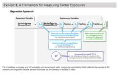
A Framework for Measuring Factor Exposures
We can use this framework to examine the exposures of a hypothetical long-only equity portfolio that aims to capture returns from value, momentum and  size style premia.³ In practice an investor may not know  the portfolio exposures in advance, but  since our goal  is to illustrate how to best apply the analysis, we will proceed as if we do.

As our explanatory variables, we use the well-known long/ short academic factors: HML, UMD, and  SMB.⁴  We use a regression model to assess drivers of portfolio returns. Specifically, we measure each factor’s contribution to portfolio returns by multiplying the factor’s beta by its respective average risk premium over the sample period (see Exhibit 2).

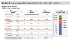
Decomposing Hypothetical Portfolio Returns by Factors                                    
The results shown in Exhibit 2 are consistent with our intuition: the portfolio had positive exposures (betas) to value (HML), momentum (UMD), and  size (SMB).⁵  And because these factors each delivered positive returns over this period, this positive exposure benefited the portfolio with value, momentum and  size contributing 2.4%, 0.5% and  1.2%, respectively, to the portfolio’s excess of cash returns.

Another important output from  Exhibit 2 is the alpha estimate, which  potentially provides insight into manager “skill.”
It’s important that investors are able to distinguish whether a manager is actually providing alpha above and  beyond their factor exposures. But doing so requires us- ing the correct model. Without the proper model, rewards for factor exposures may be misconstrued as alpha. This can lead to suboptimal investment choices, such as paying high fees for a manager that seems to deliver “alpha,” but  really  just provides simple factor tilts.

To understand this, suppose we were to look at our test portfolio against a model with the equity market as the only factor (the well-known CAPM). Against this model it would  seem that a large portion of port- folio returns are dominated by “alpha,” but as we just saw, roughly 4% of the portfolio’s returns are driven by style exposures (2.4%+0.5%+1.2%=4%). These results have important implications — if investors don’t control for multiple exposures in a multi-factor portfolio, then excess returns will look as if they are mostly alpha.

It’s also important to note that “alpha” depends on what is already in the portfolio.For any portfolio, positive expected return strategies that are uncorrelated to existing exposures can be a significant source of improvement. For example, to an investor who has passive equity market exposure, adding new  sources of portfolio returns, such as value and  momentum, will have the same effect as adding alpha to the portfolio — even if a regression containing the market, value and  momentum would explain that alpha away.⁶

Common Pitfalls  in Measuring Factor Exposures
So far we have focused on how to apply the regression framework, but  there are many pitfalls associated with regression analysis. They are nuanced and  detailed, but  they really  do matter; they relate to errors in interpretation and  factor design differences.

Errors in Interpretation

Focus too much  on betas and not on t-statistics
Many investors focus only on betas in assessing factor exposures but  fail to account for the reliability (or statistical significance) of these estimates. Just because a portfolio has a high beta coefficient to a factor doesn’t mean it’s statistically different than a portfolio with a zero beta, or no factor exposure. As such, it’s important to look at the t-statistic for each beta; a portfolio exposure that is only economically meaningful (large beta) but  not  reliable (insignificant t-statistic) could impact the portfolio in a big way, but  with a high degree of uncertainty.

Comparing betas for portfolios with different volatilities
Since volatility varies considerably across portfolios, comparisons of betas can be misleading. For the same level of correlation,  the higher a portfolio’s volatility, the higher its beta.⁷ When  investors fail to account for different levels of volatilities between portfolios, they may conclude that one  portfolio is providing more exposure than another, which  is true in notional terms — but  in terms of exposure per  unit of risk, that may not  be the case.

Failure to consider the R2 measure
The R2 measure provides insight into the overall explanatory power of the regression model; it indicates how much of the variability in returns is accounted for by the factors used. Generally, the higher the R2 the better the model is in explaining portfolio returns.

Factor Differences
In addition to the statistical issues described above, there are other questions to
consider when doing regression analysis. Investors should ask  themselves: what exactly are these factors I’m using and  are they applicable to my portfolio? The answers to these questions affect beta and alpha estimates. Factor loadings are highly influenced by the design and  universe of factors used, and  alpha estimates reflect implementation differences associated with capturing the factors. We cover these considerations in detail below.

Is the implementation comparable?
Academic factors, such as the Fama-French factors used here, do not account for implementation costs. They are gross of fees, transaction costs and  taxes. They do not  face any of the real-world frictions that implementable portfolios do. Differences in implementation approaches may be reflected in regression results. Even if a portfolio does a perfect job of capturing the factors, it could still have negative alpha in the regression model, which  would  represent implementation
differences associated with capturing the factors.⁸

Are the universes the same?
Academic factors span a wide  market capitalization range and  are, in fact, overly reliant on small-cap or even micro-cap stocks. These factors include the entire CRSP universe of approximately 5,000 stocks. Many practitioners would  agree that a trading strategy that dips  far below the Russell 3000 is not  a very implementable one, and  this is likely where most of the bottom two quintiles in the academic factors fall.

Is the portfolio long-only or long/short?
Long-only portfolios are more constrained in harvesting style premia as underweights are capped at their respective benchmark weights. In contrast, long/short factors (and portfolios) are purer in that they are unconstrained. These differences should be understood when performing and  interpreting factor analysis.

Is the portfolio based on multiple measures for each style?
Often, multiple measures can be used and applied simultaneously to form a more robust and  reliable view of a factor. For example, while stocks selected using the traditional academic book-to-price value measure perform well in empirical studies, there is no theory that says it is the best measure for value.

Does the portfolio have risk-controlled exposures?
Academic factors typically do not  have any explicit risk controls. For example, in the case of stocks, academic factors often do a simple ranking across stocks, and  in do- ing so implicitly  take style bets within  and across industries (also across countries in international portfolios), without any explicit risk controls on the relative contributions of each. In contrast, factors implemented by practitioners may differentiate stocks within  and  across industries (i.e., industry views). They are designed to capture and  target risk to both independently. As another example, practitioners also use risk targeting when constructing factors; this approach dynamically targets risk to provide more consistent realized volatility in changing market conditions. Finally, practitioners can also build market (or beta) neutral long/short portfolios, whereas academic factors are often dollar neutral, allowing for unintended, time-varying market bets.

Conclusion
Regression analysis can help investors better understand the risk factors present in their portfolios, which  has multiple benefits. It can help investors evaluate fees, by estimating what portion of returns can be attributed to systematic factor exposures versus idiosyncratic sources of return which  should command a premium. It can also lead to improved portfolio construction and  diversification, by identifying the sources of return that are missing from, and  most likely additive to, their existing portfolios.

AQR is a global investment management firm that employs a systematic, research-driven approach to manage alternative and  traditional strategies.

We manage over $141 billion for institutional investors and investment professionals.⁹
w: aqr.com

1 Style premia are sources of returns that are well researched, geographically pervasive and  have been shown to be persistent across both time  and multiple asset classes. There is a logical, economic rationale for why they provide a long-term source of return (and are likely to continue to do so). See Asness, Moskowitz and  Pedersen (2013); Asness, Ilmanen, Israel and  Moskowitz (2015); and  “How Can  a Strategy Still Work if Everyone Knows About It?,” September 23, 2015 for more information.

2 For more information on measuring portfolio factor exposures, see Israel and  Ross (2015). 

3 The portfolio is constructed with 50/50 weight on simple measures of value (book-to-price, using the Asness and  Frazzini (2013) HML Devil methodology of current prices) and  momentum (12 month price return, skipping the most recent month) within  the small-cap universe. 

4 For simplicity, we use academic factors, instead of practitioner factors, sourced from  Ken French’s data library. HML is a portfolio that goes long stocks with high book-to-market values and  short stocks with low book-to-market values; UMD goes long stocks with high returns over the past 12 months (skipping the most recent month) and  short stocks with low returns over the same period; SMB goes long small-market-cap stocks and  short large-market-cap stocks. 

5 Note that if we were to use HML Devil (using current prices) instead of HML (using lagged prices) we would  see a higher loading on UMD. See Israel and  Ross (2015) and  Asness and  Frazzini (2013) for more information on how HML can be viewed as an incidental bet on UMD, which  affects regression results by lowering the loading on UMD (as HML is eating up some of the UMD loading that would  otherwise exist). 

6 Berger, Crowell, Israel and  Kabiller (2012). 

7 Based on a univariate regression. 

8 Note that our hypothetical portfolio is also gross of fees, transaction costs and  taxes, which  makes the use of academic factors in the analysis less problematic (compared to looking at a live portfolio that faces real  world  frictions). 

9 As of December 31, 2015. 

The information set forth herein has been obtained or derived from  sources believed by AQR Capital Management, LLC (“AQR”) to be reliable. However, AQR does not  make any representation or warranty, express or implied, as to the information’s accuracy or completeness, nor does AQR recommend that the attached information serve as the basis of any investment decision. and  does not  constitute an offer or solicitation of an offer, or any advice or recommendation, to purchase any securities or other financial instruments, and  may not  be construed as such. AQR hereby disclaims any duty to provide any updates or changes to the analyses contained in this article. 

The data and  analysis contained herein are based on theoretical and  model portfolios and  are not  representative of the performance of funds or portfolios that AQR currently man- ages. There is no guarantee, express or implied, that long-term volatility targets will be achieved. Realized volatility may come in higher or lower than expected. Past performance is not a guarantee of future performance.

Hypothetical performance results (e.g., quantitative backtests) have many inherent limitations, some of which, but  not  all, are described herein. No representation is being made that any fund  or account will or is likely to achieve profits or losses similar to those shown herein. In fact, there are frequently sharp differences between hypothetical performance results and  the actual results subsequently realized by any particular trading program. One  of the limitations of hypothetical performance results is that they are generally prepared with the benefit of hindsight. In addition, hypothetical trading does not  involve financial risk, and  no hypothetical trading record can completely account for the impact of financial risk in actual trading. For example, the ability  to withstand losses or adhere to a particular trading program in spite of trading losses are material points which  can adversely affect actual trading results. The hypothetical performance results contained herein represent the application of the quantitative models as currently in effect on the date first written above and  there can be no assurance that the models will remain the same in the future or that an application of the current models in the future will produce similar results because the relevant market and  economic conditions that prevailed during the hypothetical performance period will not  necessarily recur. There are numerous other factors related to the markets in general or to the implementation of any specific trading program which  cannot be fully accounted for in the preparation of hypothetical performance results, all of which can adversely affect actual trading results. Discounting factors may be applied to reduce suspected anomalies. This backtest’s return, for this period, may vary depending on the date it is run. Hypothetical performance results are presented for illustrative purposes only.

There is a risk of substantial loss associated with trading commodities, futures, options, derivatives and  other financial instruments. Before trading, investors should carefully con- sider their financial position and  risk tolerance to determine if the proposed trading style is appropriate. Investors should realize that when trading futures, commodities, options, derivatives and  other financial instruments one  could lose the full balance of their account. It is also possible to lose more than the initial deposit when trading derivatives or using leverage. All funds committed to such a trading strategy should be purely risk capital. © AQR Capital Management, LLC. All rights reserved.